


3.1.1 What is a climate model ?
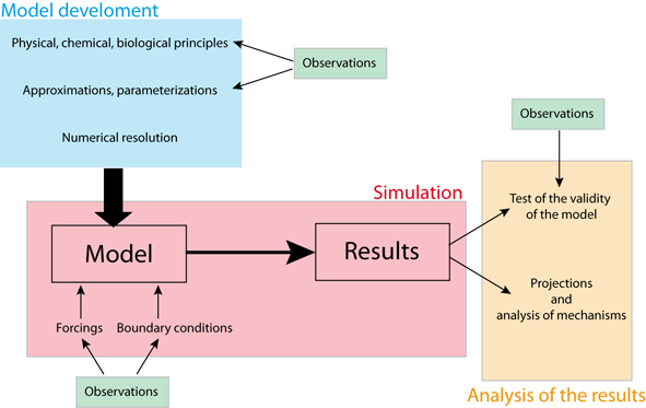
In general terms, a climate model could be defined as a mathematical representation of the climate system based on physical, biological and chemical principles (Fig. 3.1). The equations derived from these laws are so complex that they must be solved numerically. As a consequence, climate models provide a solution which is discrete in space and time, meaning that the results obtained represent averages over regions, whose size depends on model resolution, and for specific times. For instance, some models provide only globally or zonally averaged values while others have a numerical grid whose spatial resolution could be less than 100 km. The time step could be between minutes and several years, depending on the process studied.
Even for models with the highest resolution, the numerical grid is still much too coarse to represent small scale processes such as turbulence in the atmospheric and oceanic boundary layers, the interactions of the circulation with small scale topography features, thunderstorms, cloud microphysics processes, etc. Furthermore, many processes are still not sufficiently well-known to include their detailed behaviour in models. As a consequence, parameterisations have to be designed, based on empirical evidence and/or on theoretical arguments, to account for the large-scale influence of those processes not included explicitly. Because these parameterizations reproduce only the first order effects and are usually not valid for all possible conditions, they are often a large source of considerable uncertainty in models.
In addition to the physical, biological and chemical knowledge included in the model equations, climate models require some inputs derived from observations or other model studies. For a climate model describing nearly all the components of the system, only a relatively small amount of data is required: the solar irradiance, the Earth's radius and period of rotation, the land topography and bathymetry of the ocean, some properties of rocks and soils, etc. On the other hand, for a model that only represents explicitly the physics of the atmosphere, the ocean and the sea ice, information in the form of boundary conditions should be provided for all sub-systems of the climate system not explicitly included in the model: the distribution of vegetation, the topography of the ice sheets, etc.
Those model inputs are often separated into boundary conditions (which are generally fixed during the course of the simulation) and external forcings (such as the changes in solar irradiance) which drives the changes in climate. However, those definitions could sometimes be misleading. The forcing of one model could be a key state variable of another. For instance, the changes in CO2 concentration could be prescribed in some models while it is directly computed in models including a representation of the carbon cycle. Furthermore, a fixed boundary in some models, like the ice sheet topography, can evolve interactively in a model designed to study climate variations on a longer time scale.
In this framework, some data are required as input during the simulation. However, the importance of data is probably even greater during the development phase of the model, as they provide essential information on the properties of the system that is being modelled (see Fig. 3.1). In addition, large numbers of observations are needed to test the validity of the models in order to gain confidence in the conclusions derived from their results (see section 3.5.2).
Many climate models have been developed to perform climate projections,
i.e. to simulate and understand climate changes in response to the emission of
greenhouse gases and aerosols. In addition, models can be formidable tools to
improve our knowledge of the most important characteristics of the climate system
and of the causes of climate variations. Obviously, climatologists cannot perform experiments
on the real climate system to identify the role of a particular process clearly or to test a
hypothesis. However, this can be done in the virtual world of climate models. For highly
non-linear systems, the design of such tests, often called sensitivity experiments, has
to be very carefully planned. However, in simple experiments, neglecting a process
or an element of the modelled system (for instance the influence of the increase in
CO2 concentration on the radiative properties of the atmosphere)
can often provide a first estimate of the role of this process or this element in the system.